Description
This
test case is provided for you to check your code before
running the assigned problem for Problem 4.
Please note the settings below, and remember to change all
settings back to the official problem(s) before running
and handing in results.
- Grid layout: 201x41; ∆x=∆z=100 meters
- Quasi-compressible sound speed Cs = 100 meters/sec
- Integration: time step ∆t = 0.25 sec; run for 2400 steps (T=600s)
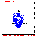
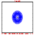
- This test includes full physics, with the initial condition U = W = P' = 0, and T' = a cool bubble in the domain center.
- Initial bubble location: center (10050, 2050) meters, which is grid point (101,21).
- Initial bubble specification: center perturbation magnitude -15 °C, "radii" in X: 4000 m; Z: 1000 m.
- Diffusion: done for all k=[1,...,nz] for U and Theta
- Diffusion coefficient = 50.0 (for U, W) for all cases; diffusion for theta = 40.0 (for all, Lax-W and PL)
- Results are included below for different
advection options (Lax-Wendroff and Piecewise
Linear with and without monotonic slopes)
- >>> These results had theta diffusion evaluated at time (n) -=> we will do this at (n-1), so these results are no longer correct for our use, expect some differences <<<
Test case results
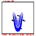
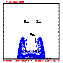
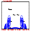
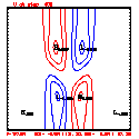
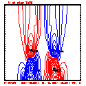
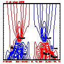
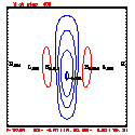
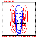
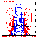
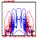
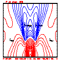
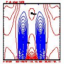
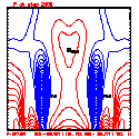
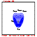
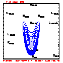
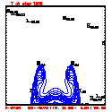
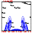
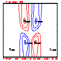
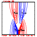
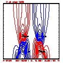
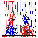
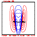
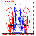
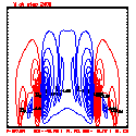
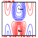
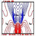
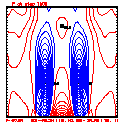
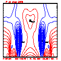
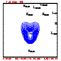
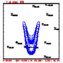
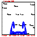
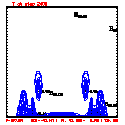
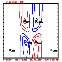
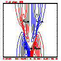
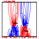
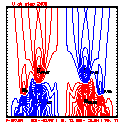
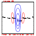
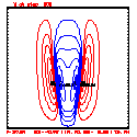
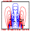
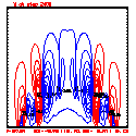
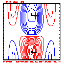
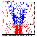
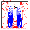
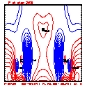
- Plots below use contour intervals of 2.0 (for U and W), 1.0 (for Theta'), and 25.0 (for P').
- Partial text output from these runs: Lax-Wendroff,
Piecewise
linear (non-monotonic),
Piecewise
linear (monotonic)
- Multi-image viewer web pages:
First 50 steps / Full runs:
Lax-Wendroff /
PL (non-monotonic) /
PL (monotonic)
these viewer web pages self-size to fill the window; stretch the browser window to fill your screen to get the largest images
- Thoughts about these solutions:
- Piecewise linear (PL) looks better. Smoother. There is more implicit damping! It looks better, but is it?
- Realistically we could - and should - run less explicit diffusion when using PL than with Lax-Wendroff.
- Using the monotonic slope limiter with PL means that the theta' max stays near zero, at the cost of extra diffusion. Compare the final (2400 step, 600s) plots of theta' for PL vs. monotonic-PL.
- If you look carefully at the every-step-plotted Lax-Wendroff results, you'll see something oscillating every other time step. I'm guessing this is due to the Leapfrog computational mode, and it would go away with time smoothing.
- If you like how Piecewise Linear works for your own research, you should consider piecewise parabolic for even higher accuracy, with less implicit diffusion.

