Updated - Sun. Mar. 23
Description
Rotational flow test
case results:
Settings for test case:
Description
- Problem: Linear advection, rotational flow, with moving nested grid.
- Method: Lax-Wendroff (only), with automatic grid
nest placement (but fixed nested grid size)
- Official program settings: TBA (use test case settings for now - see below)
- Output: For this program, you are required to use my make-web-pages script(s) to make images and web pages, in addition to the usual "these particular plots" results. See below.
- Due date: TBA
- Problem handout: PDF
Takacs Error calculations for Program 3 (and 2)
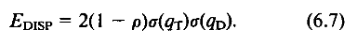
Some of this was in the program #2 page.- I used Takacs' error equations 6.1, 6.6, and 6.7:
- Total error:
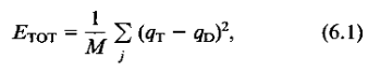
- Dissipation:

- Dispersion :
- Total error:
- For Takacs' equations, I used the
sample (biased) variance;
remember to take the square root to get the
standard deviation σ that appears in equations 6.6 and 6.7. - For the correlation coefficient ρ I used the Pearson formula.
Web pages & shell scripting for Program 3
Creating web pages:- Copy
(cp)
my files on Keeling:
cp ~bjewett/502/Web/* .
(don't omit the
dot at the end of this command!)
- to Linux, the dot here means: copy those files to my current (".") directory without changing any file names
- To use these scripts:
- Copy those files to your Program3 directory containing a 'gmeta' plot file.
- Figure out the first plot frame number (1=first plot, 2=second..) where your plots start following a regular sequence, e.g. truncation error, coarse S1, nest S1 ... then next data time
- Edit make_images on Keeling (it is just a text file, so nano or vim works), and change first_plot to refer to that first plot (e.g. skipping IC fields), and change plot_names to whatever you want to call your plot sequence (no spaces allowed in names!)
- Run: make_images ... or if the plot file isn't gmeta: make_images name-of-plot-file
- Run: make_viewer zip
- Send the .zip file containing plots & .shtml files to your PC, unzip, and open with a browser
- in some cases it won't open correctly when you just double-click the file ... if that happens, try opening the file directly from your browser with control-O (on a mac, use command key: ⌘-O)
- Here is the web page I got from running it on my demo plot file, gmeta_Brian: viewer2p.shtml
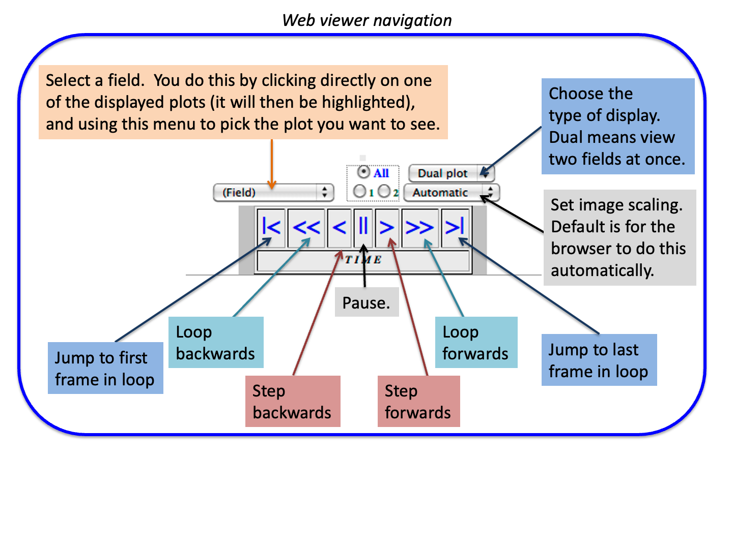
- To navigate/use the resulting web pages:
- See this: Web viewer explanation image
- You can choose to view 2-, 4-, 6- images at once with "Dual plot" menu button
- You can choose which plot appears in which image place using the (Field) menu button
- My main Shells + scripting page
- My latest 'run' script is on Keeling at: ~bjewett/502/Pgm3/run
- The run script (also also here) has the following sections:
- Settings: set your email address here, as well as the name of the running program e.g. pgm3
- Deletes old files (to make sure you don't run an old version or view old, outdated plots)
- Builds the code with make, and stops if there was a problem.
- Runs the program
- It uses the Linux tee command to both send output to a file, and to your screen.
- Plots the results in either or both of two ways:
- using idt
- Emailing you the text output plus a zip file of the gmeta file, as .GIFs
- It would be easy to add the 'build web pages' steps here too.
Nesting and plot routines for Program #3
The following are provided to you. They are available- on Keeling in ~bjewett/502/Pgm3/C or ~bjewett/502/Pgm3/Fortran
- demo dointerp
code compile instructions: C
programmers / Fortran
dointerp handles
interpolation between the coarse and nested grids;
feedback; and nested grid boundary conditions
nestwind provides the nested grid analytical wind field, given the nest location in coarse grid coordinates
test_interp a short program showing you how to call dointerp to set BCs, create a "nest", and do feedback.
README -- describes how to compile the test_interp program.
nestwind provides the nested grid analytical wind field, given the nest location in coarse grid coordinates
test_interp a short program showing you how to call dointerp to set BCs, create a "nest", and do feedback.
README -- describes how to compile the test_interp program.
How to get program 3 started/working!
- Make a copy of your directory for program 2 (e.g.: cp -R pgm2 pgm3)
- In your main program, you will need some extra nesting variables - see below.
- Place the nest using the initial condition field:
- Make sure your grid parameters correspond to the program 3 test case! (farther down on this page)
- After calling IC() and plotting the (coarse grid) initial conditions (s1, u, and v):
- Call your routine to compute the truncation error (TE). Until everything is working, I suggest also calling contr() to plot the TE array.
- Once you have the TE computed, compute the grid-point-flagging criteria (half the TE array max value)
- Find the left-right-bottom-top edges of the "more than criteria" region, then average to find the center location of the nest. Print out this nest center location.
- Find the left-right-bottom-top edges of the NEST - not to be confused with the edges of the
truncation error points. Remember in our case the nest could be smaller or larger than
the region of large truncation error. To find the nest edges, I:
- Compute nestsize = (nx-1)/refinement_ratio
- nestX1 = nest_x_center - nestsize/2
- nestX2 = nestX1 + nestsize
- nestY1 = nest_y_center - nestsize/2
- nestY2 = nestY1 + nestsize
- Make sure your nest location doesn't run off an edge of the coarse grid --- this means:
- In Fortran, that nestX1 >= 1 and nestX2 <= nx and nestY1 >= 1 and nestY2 <= ny (in C, use i1,i2,j1,j2)
- If for example it is crossing the top edge of the domain, then nestY2 is > ny. Fix by setting nestY2 = ny, and nestY1 = nestY2 - nestsize
- call dointerp to place the nest (fill up s1nest values from s1coarse grid)
- call contr to draw contours for your nested grid array that dointerp filled in
with interpolated coarse-grid values.
If the nest is centered and called OK, you'll see a "cone" at the nest center - and appearing much larger than on the coarse grid. - call contr to draw contours for your coarse grid again, but this time with the nested grid coordinates (instead of 0,0,0,0) in the call to contr(). You should see your coarse grid cone, with the nested grid boundaries shown in red.
- call nestwind to fill up the unest and vnest arrays - and plot u(nest) and v(nest), too.
- call the close-ncar-graphics routines at the bottom of the code and stop (in C, exit(0)). Focus on getting the nest position OK before going any farther!
- Add nest-movement code at the start of (but inside) your main time-step loop:
- If the time step is a multiple of the required interval (test case: every 5 steps) ...
- If you haven't already, save your nestX1, nestX2, ... in old-nest variables (e.g. nestX1old)
- Call your TE routine to find the new nest center
- Compute the new nest edges: nestX1, nestX2, ... etc.
- Move the nest from the old to new location by calling dointerp()
- Update the unest, vnest arrays by calling nestwind()
- If the time step is a multiple of the required interval (test case: every 5 steps) ...
- Continue your steps inside the main time step loop:
- call bc (for the coarse grid)
- call dointerp (to set BCs for the nested grid)
- call advection (for the coarse grid)
- Inside a new loop: call advection for the nest multiple times
- Perform feedback by calling dointerp (only if feedback is turned on!)
Calling dointerp:
See the test_interp routine in the Fortran or C
directory for examples of how to call dointerp
and nestwind.
In Fortran, you call dointerp routine in this
way:
call dointerp(q1,
q1nest, nx,ny, bcwidth, nestX1, nestX2, nestY1, nestY2
n,ratio,flag, nestX1old, nestX2old, nestY1old,
nestY2old)
- q1 - name
of the coarse grid. Pass the whole array -
including ghost points - to dointerp.
- q1nest - name of
the nested grid. Pass the whole array -
including ghost points - to dointerp.
- nx,ny -
dimensions of the grid (not including ghost points
for Fortran) (so this really IS just nx,ny)
- bcwidth - number of ghost points
you are using.
- nestX1 ... nestY2 - four integers defining the nest position -
- IF you are first placing the nest
OR you are setting nest BCs OR
you are doing feedback,
then these four integer variables define the current position of the nest on the coarse grid ...
and the variables nestX1old,nestX2old,nestY1old,nestY2old are ignored by dointerp.
- IF you are moving the nest, these
are the (future) coordinates of where
the nest should be moved, and
nestX1old,nestX2old etc. define the current position of the nest on the coarse grid. - n
- the time step counter, used by print statements
inside the routine. Pass 0 if you wish.
This is an integer.
- ratio - nest refinement factor, an integer such as 3
- flag - a key variable (an integer) telling dointerp what to do.
- when flag = -1, dointerp will move the nest, from old (nestX1old, etc.) to new (nestX1, etc) positions
- when flag = 1, dointerp will place the nest: interpolate coarse > nest. We do this only once.
- when flag = 10, dointerp will set nested grid boundary values. Nest interior values are unchanged.
- when flag = 2, dointerp will do
feedback - to the coarse grid from the
nest.
- nestX1old...nestY2old are ignored except in the case when the nest is being moved.
- When the nest is being moved, nestX1old
... nestY2old are the current (soon to be old!)
position of the nest,
and the variables nestX1 ... nestY2 contain the new nest position you want. - When calling dointerp for cases other
than moving the nest, just pass 0,0,0,0
for these four variables.
Rotational flow test
case results:
Settings for test case:- 106x106 grid
- Domain [-0.5, +0.5] as before
- Cone width is 0.075
- Nest time/space refinement ratio = 3
- Nest moved every 5 time steps
- Run 360 steps; Time step = pi / 360
Results for test case:
These plots use my simulation viewer web pages -
click for instructions on using pages
| Initial condition | No feedback | With feedback |
| First 40 steps, only | plots, text | plots (2-panel), plots (8-panel), text |
|---|---|---|
| Full rotation | plots, text | plots (2-panel), plots (8-panel), text |