Updated
Wed. Feb. 25
~bjewett/502/Pgm2
There are also options to create movies (animated GIFs or Quicktime) in the script metagif. For more information, try
~bjewett/502/Tools/metagif -help
For more information on how to use the simple contr() and sfc() routines for 2-D plotting in program 2, see this web page.
There are also files in my Pgm2 directory regarding making of web pages to display your data - this will be discussed in class.
Test results to evaluate your code
Note the differences between the test parameters
and your assignment.
>> Be sure to change all these parameters back to the official problem before running & handing your results in!
Description
- Problem: 2-D linear advection via fractional step (directional) splitting
- Flow field: rotational flow (counter-clockwise), constant w/time.
- Methods
- Lax-Wendroff (from program 1),
- Takacs (see PDF for details), and
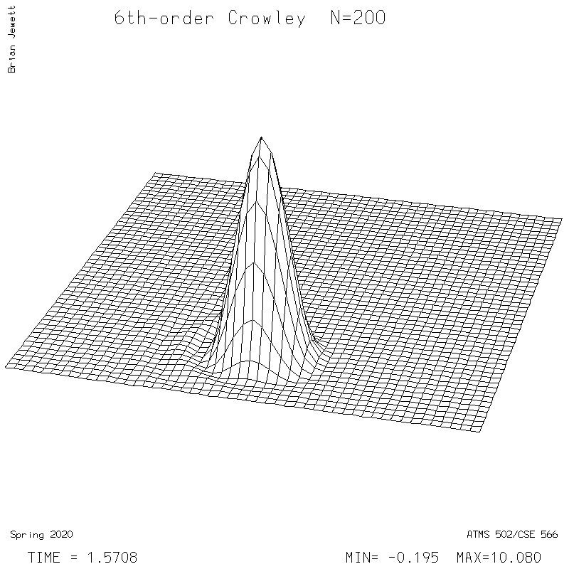
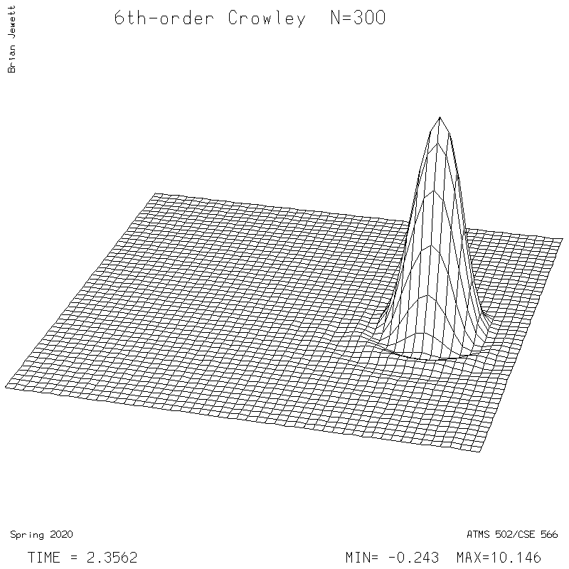
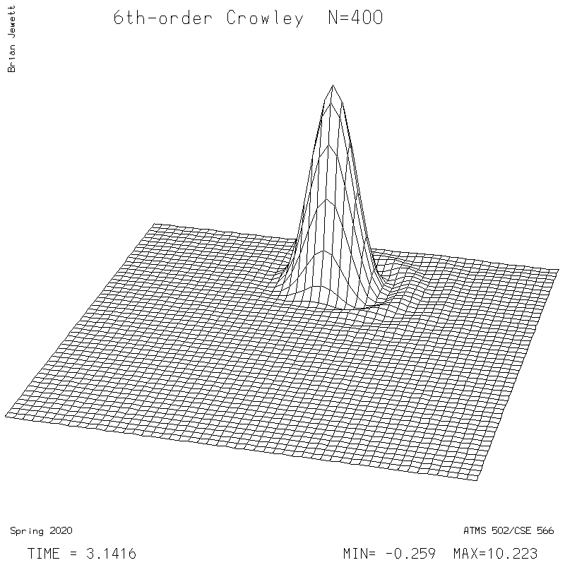
- 6th-order Crowley -- scheme available from Tremback (1987), PDF page 542, equation "ORD=6".
- Boundary conditions: 0-gradient in both directions (ghost point values = nearest edge value)
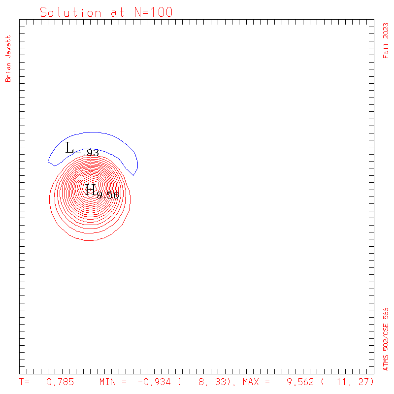
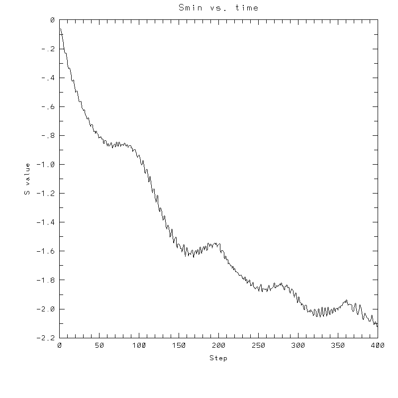
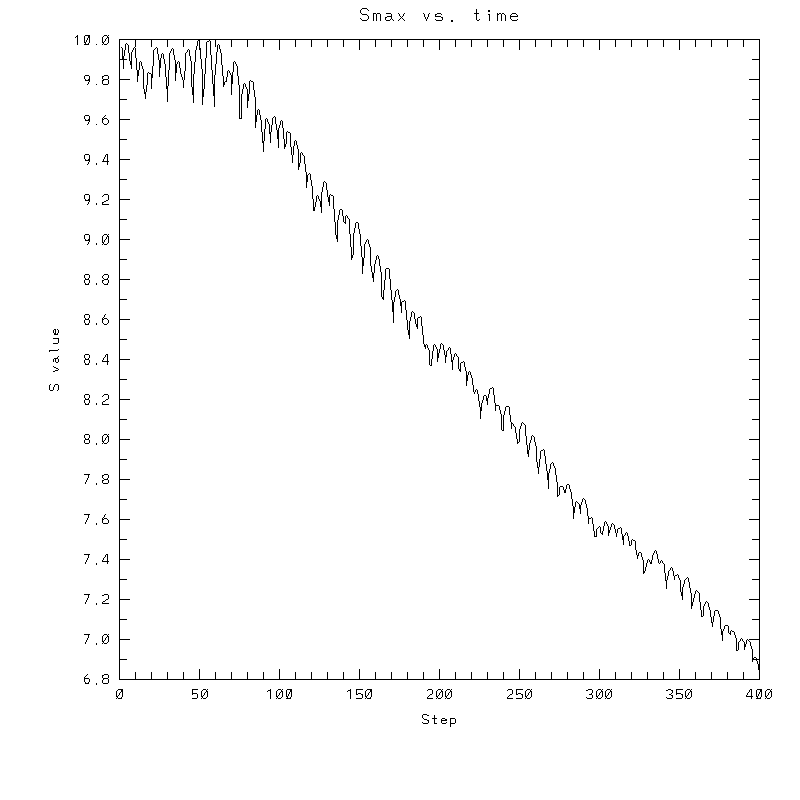
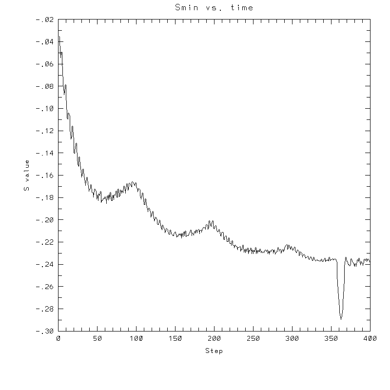
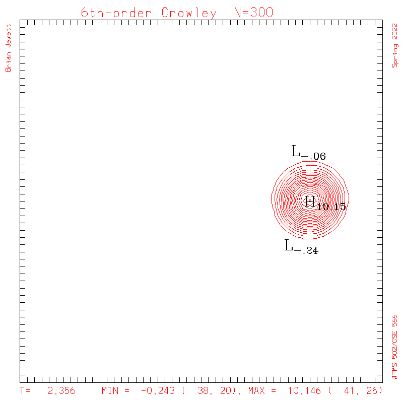
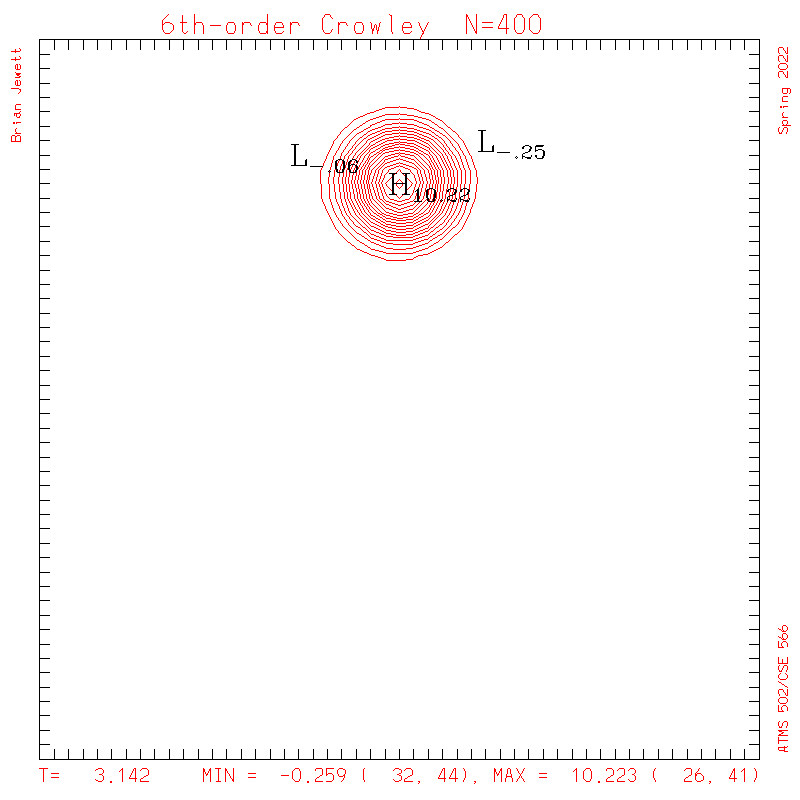
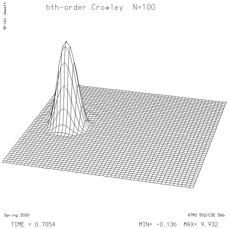
- Evaluation: Compute Takacs (1985) error statistics (eq. 6.1, 6.6, 6.7) over the entire 2-D domain after integration completed. The initial condition is the exact solution for the final time. I used sample (biased) variance, and Pearson's correlation coefficient. I provide error stats for the test case results below.
- Plan of attack: Get things working for Lax-Wendroff first. If you have difficulties,
try running your code with everywhere
- (a) U=1.0 and V=0 [cone should move to right], and then
- (b) U=0.0 and V=-1 [cone should move downward].
- FAQ/Questions+Answers section is at the bottom of this page.
- C programmers:
- be careful with array dimensions. I suggest passing NXDIM,NYDIM in your calls to subroutines, so you can define them in the routines as e.g. s1[][nydim]. With two ghost points, your s() arrays are nx+4,ny+4 points - to avoid confusion, don't hardcode the dimensions as e.g. nx+2; this is why NXDIM, NYDIM are used. Of course, you can use an include statement instead of passing parameters like NXDIM.
- watch your u,v indices in advection. For s1 or s2, you use array index limits i1,i2,j1,j2. For U and V, there are no ghost points, so you probably will use a separate array index or statements with e.g. [i-i1]. Contact me with questions.
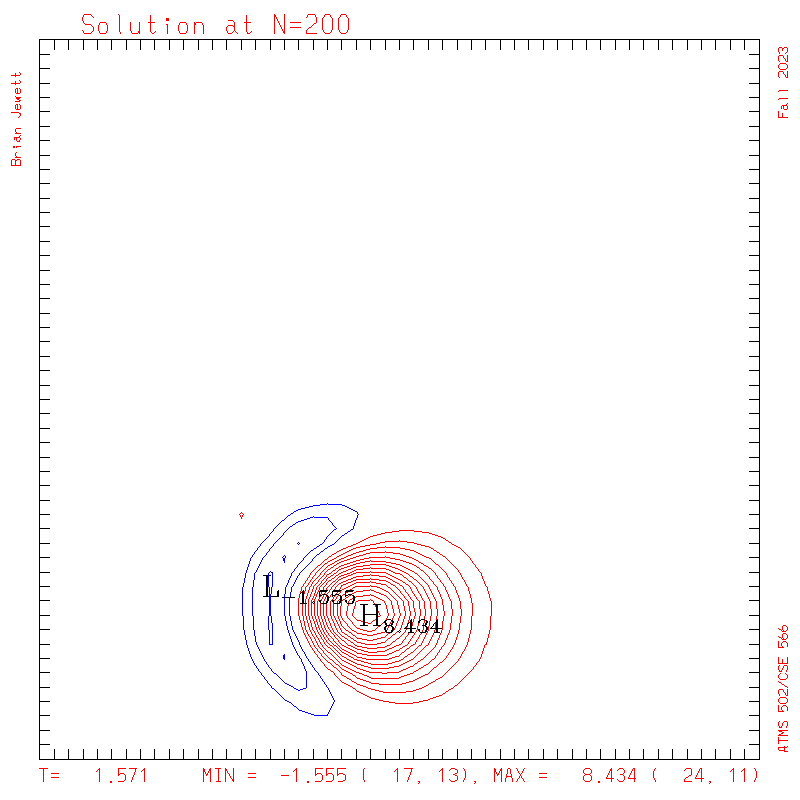
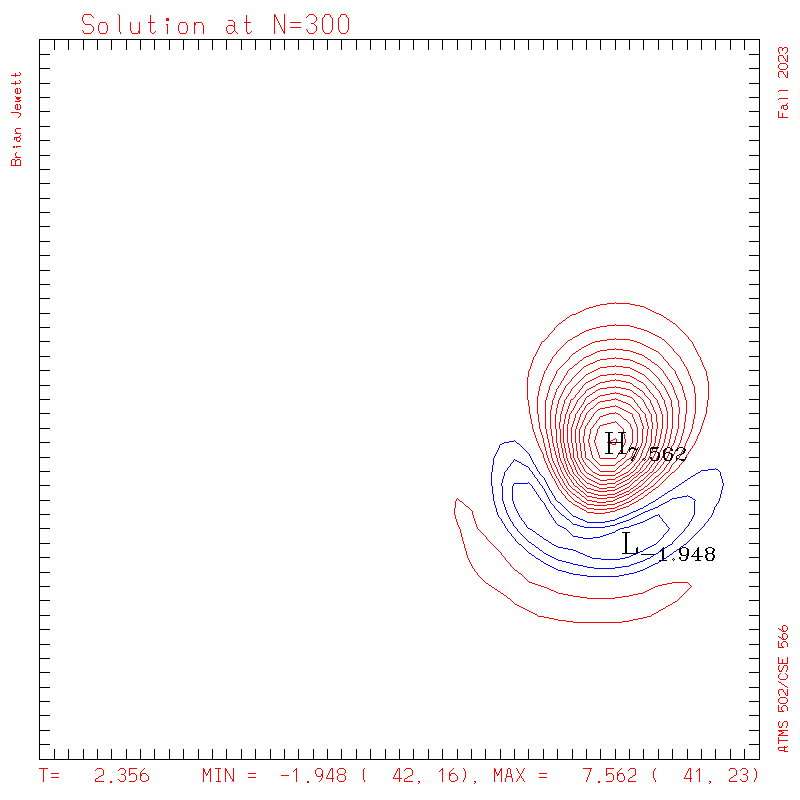
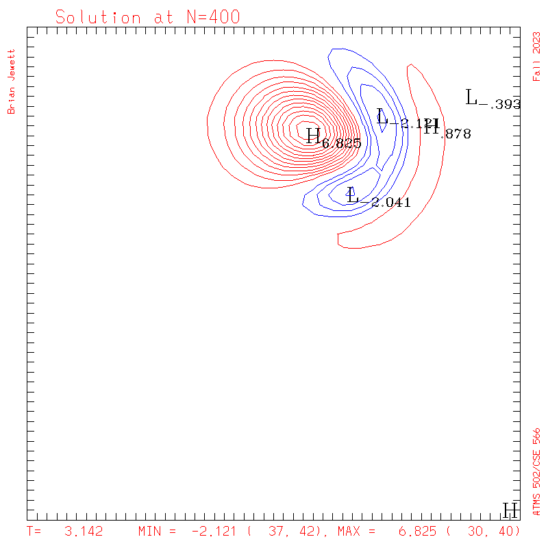
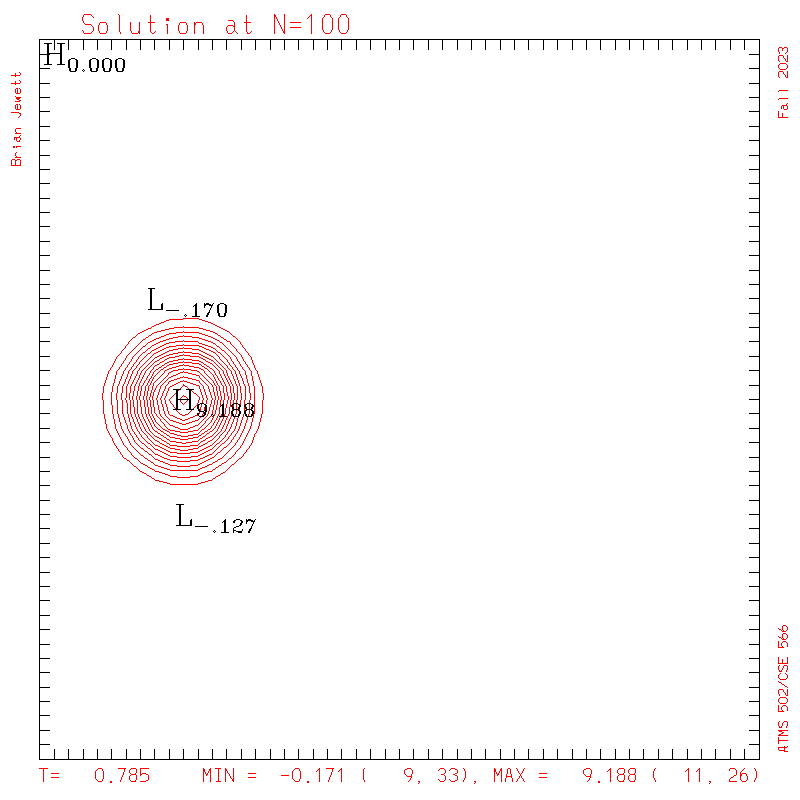
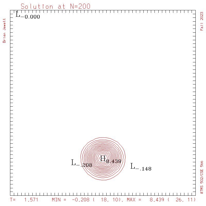
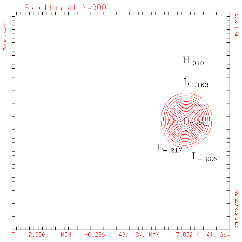
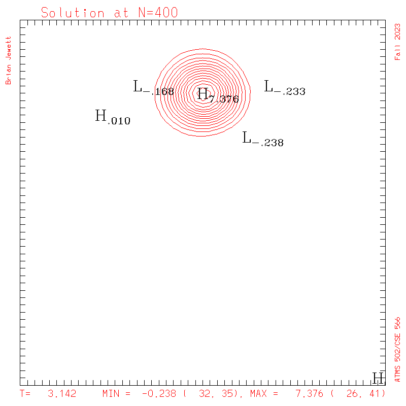
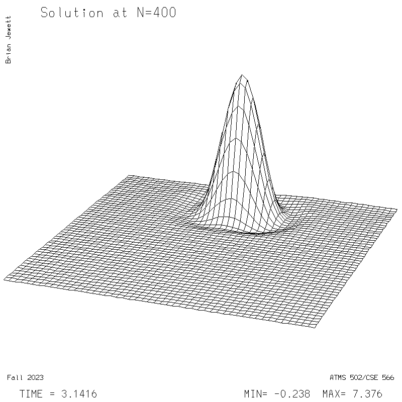
- Contour intervals: In my plots below I used a contour interval of 0.5 -- not 1.0 -- for the scalar "s" field !!
- No History required: There is no need to create time-space "history" plots in program 2. So please delete the history() array declaration and the nested do- (or for-) loops used to fill in history() as we did in program 1.
- All: if your 1-D [ezy()] plots look blank - please DELETE any agsetf calls leftover in your code from program #1. Those were appropriate for our program 1 sine function, whose data range was about -1.2 to 1.2 ... but here our 'cone' values start out between [0,10]. Leaving the agsetf() calls out lets ezy pick the scales, which is just fine here.
Test programs to show how to plot 2-D fields in Program #2
You are asked to produce contour and (optionally) surface plots for this program. Instructions are here. I have placed test programs to show how to call my contr and sfc, for plotting contours or surfaces, from C or Fortran, on Keeling at this location:~bjewett/502/Pgm2
There are also options to create movies (animated GIFs or Quicktime) in the script metagif. For more information, try
~bjewett/502/Tools/metagif -help
For more information on how to use the simple contr() and sfc() routines for 2-D plotting in program 2, see this web page.
There are also files in my Pgm2 directory regarding making of web pages to display your data - this will be discussed in class.
Test results to evaluate your code
Note the differences between the test parameters
and your assignment.>> Be sure to change all these parameters back to the official problem before running & handing your results in!
Settings:
- Note this test case
used different settings from the official hand-in
problem!!
- Domain is 51x51
- Cone size (radius) was 0.120, unlike value in the hand-in problem.
- These will be updated -- check back soon.
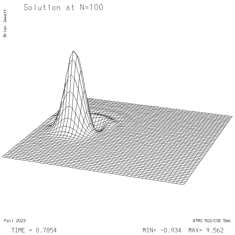
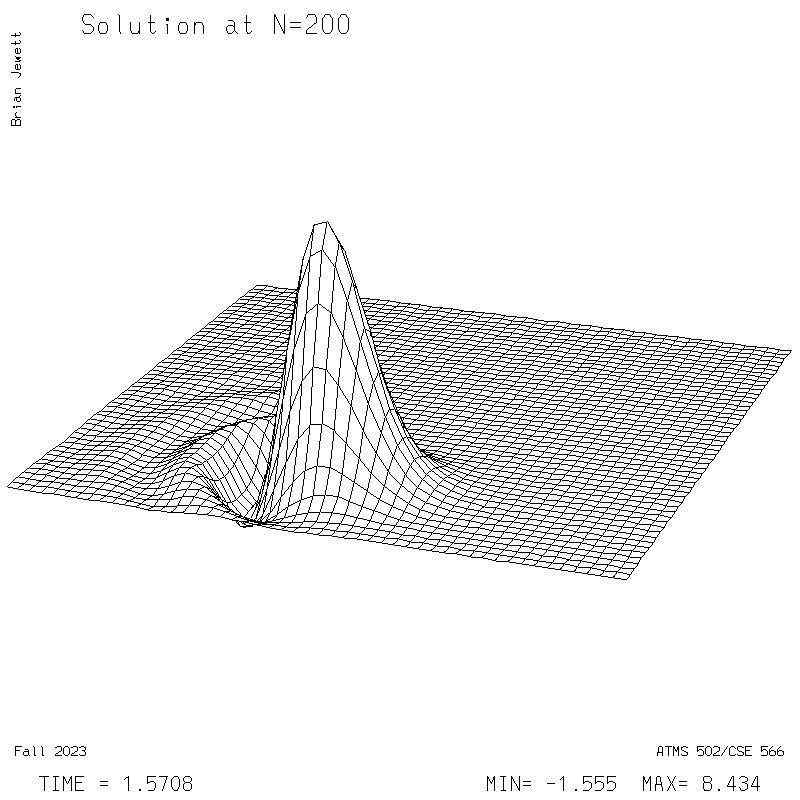
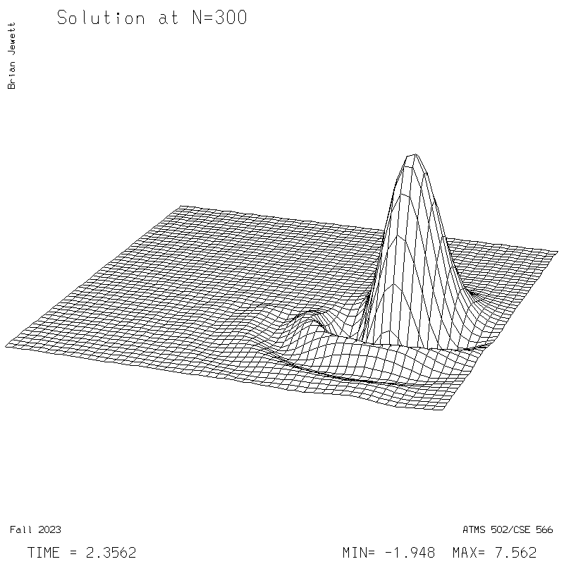
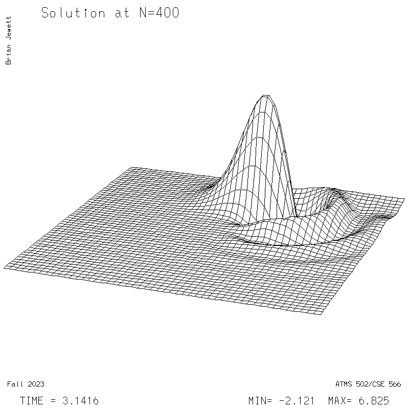
- I plotted every 100 steps. I show both contours and surface plots below.
- INITIAL CONDITION
plots: (scalar field contour interval = 0.5; U/V
contour interval = 0.1)
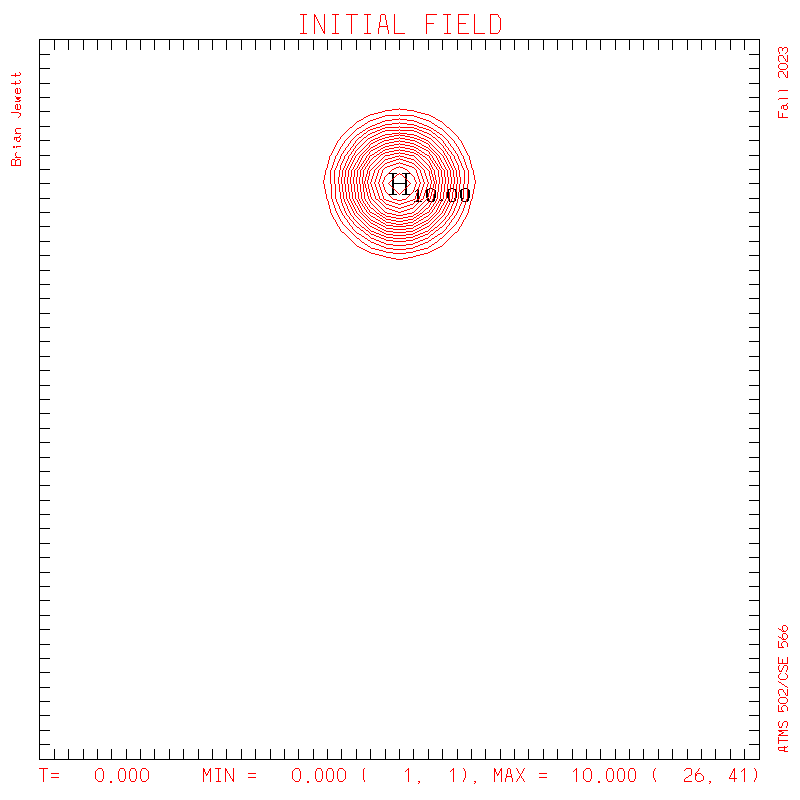
S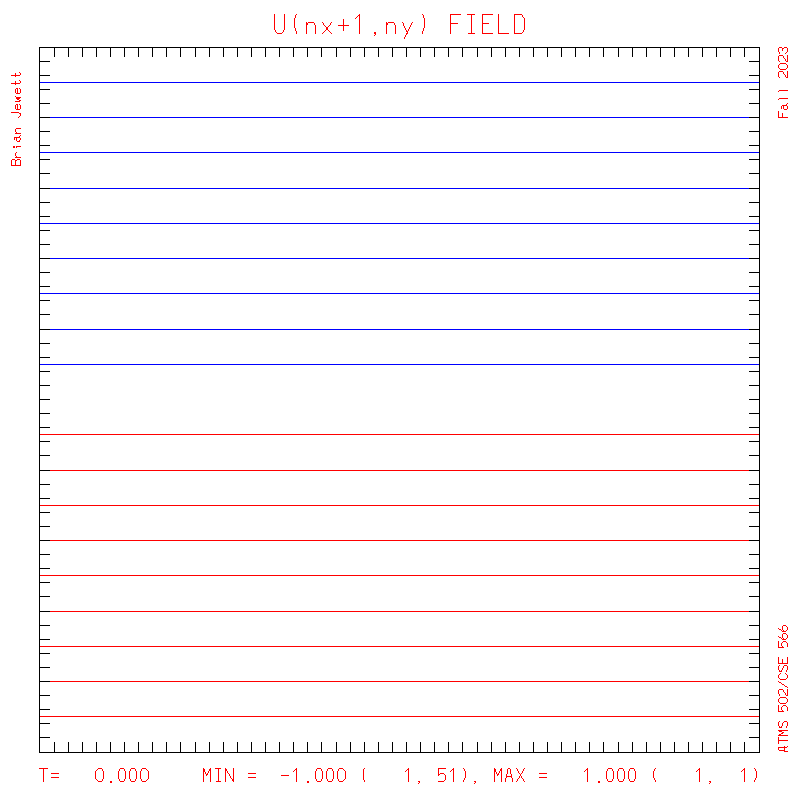
U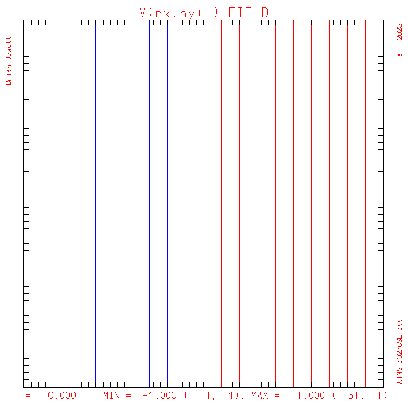
V - Test case plots:
- To answer several questions: your error stat results need not match mine exactly, but the contour plots should be very similar to mine, and the stats should probably agree to 3 decimal places, and the dispersion + dissipation error should equal your total error.
- Note: my contour interval for the scalar field is 0.5 ... but the contour interval for U,V is 0.1
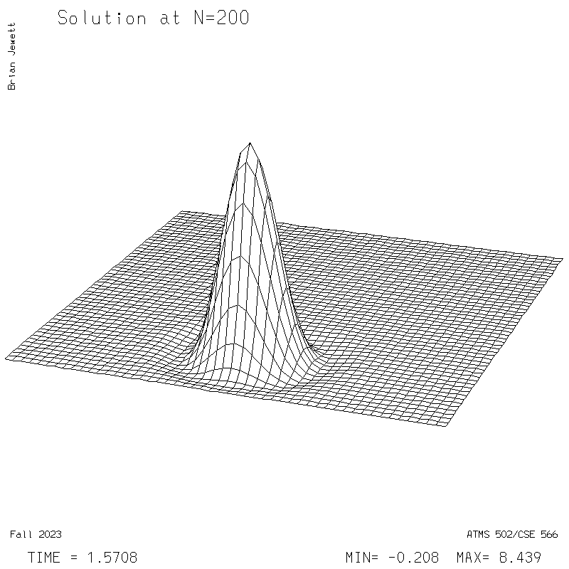
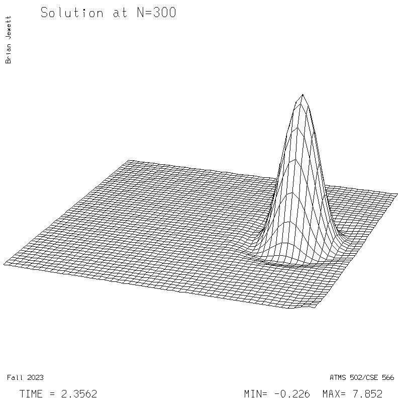
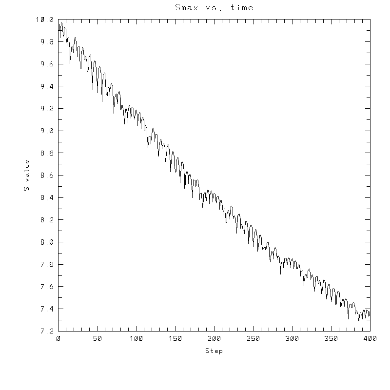
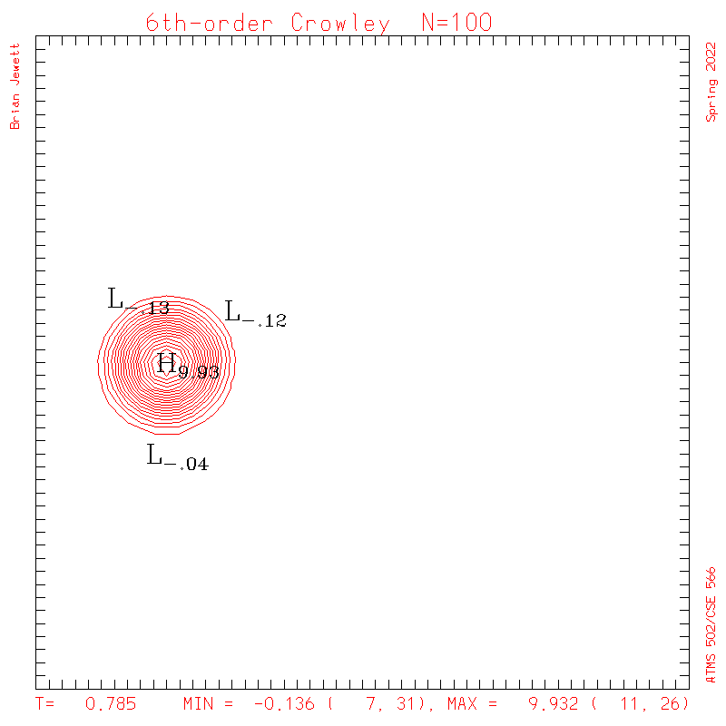
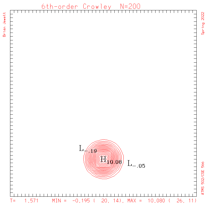
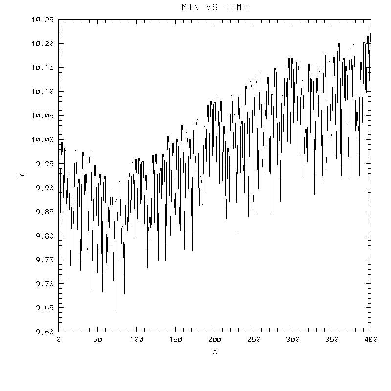
| Test case | N=100 | N=200 | N=300 | N=400 (1 cycle) | Min/max plots |
|---|---|---|---|---|---|
| Lax-W contours |
 |
 |
 |
 |
 |
| Lax-W surface |
 |
 |
 |
 |
 |
| Takacs contours |
 |
 |
 |
 |
 |
| Takacs surface |
 |
 |
 |
 |
 |
| Crowley 6th contours |
 |
 |
 |
 |
 |
| Crowley 6th surface |
 |
 |
 |
 |
 |